Introduction
Color plays a crucial role in film, impacting visual storytelling, atmosphere, tone, branding, and context. It can evoke emotions, set the mood, and emphasize the message’s theme. Therefore, mastering color is vital for filmmakers. Films can become memorable through the emotions they evoke and the symbols they express based on their color choices.
While shot detection in films is relatively straightforward using image classification models, scene detection, which involves identifying a collection of shots or frames, is more challenging. Existing models struggle with this task. An algorithm called ShotCol is one attempt at scene boundary detection, but it falls short when frames overlap between scenes.
In this study, we explore a novel approach to scene detection in films using chromatic analysis. Our focus is on two main tasks: creating a method to identify the time frame of specific frames in a film based on their average RGB values and determining the movie from which a frame originates. This research has practical applications in video search and retrieval.
 Figure 1: Suppose given a clip/video as a query, we try to identify the film it originates from and the timeslot.
This research was inspired by Tommaso Buonocore’s work, adding machine learning and genomic data science capabilities. You can find more information in his write-up, Part 1 and Part 2. We initially attempted to use Buonocore’s R package, chromaR, and its movie database but encountered issues with dependencies. Therefore, we approached Part 1 with some modifications.
While pattern-matching tools like grep or regex are typically used for such tasks, our project prioritized closeness over exactness.Pattern matching tools like regex focus on exact matches, whereas in sequence alignment, a scoring matrix assesses closeness by considering matches, mismatches, and gaps. This approach allows for the inclusion of noise during data extraction and transformation, which aligns with the project’s objectives.
Extraction
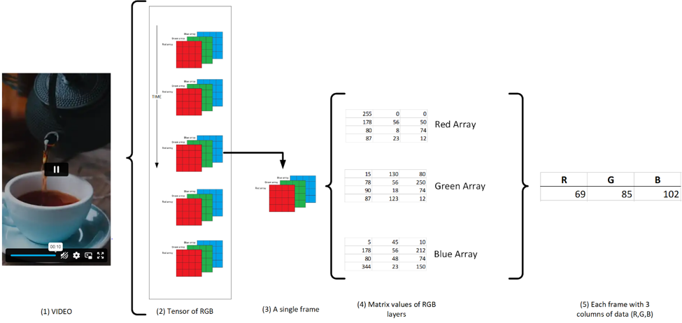
The data, consisting of RGB values, were extracted from all the frames from a video/film. As the video/film gets longer, so does the amount of frames required to be extracted. For example, a video at 24 frames per second (fps) with a length of one hour will contain 86,4000 frame layers. Hence, the reason videos/films take considerable storage. Next, as each frame contains three arrays of RGB for each pixel (subpixels), the average was calculated to represent the whole frame as shown in Figure (2). The method used Tommaso Buonocore code for extraction:
 Figure 2: A sample clip consists of multiple frames. For each frame, the RGB arrays are averaged, creating 3 columns of values required for our project.
Transformation
After extracting RGB values for each frame from the source, we applied a transformation to reduce the number of rows, as many frames are redundant or nearly identical. Figure 3 (C) illustrates that frame variability is generally low between neighboring frames unless there’s a significant change in the setting or scenes. To simplify the process, we assumed a constant frame rate of 25 fps, which is typical for films. By multiplying this frame rate by a predefined capture rate (e.g., 5 seconds), we determined the number of frames to be averaged. For instance, in a video with 851 frames, setting a 5-second capture rate at 25 fps would result in 125 consecutive frames being averaged together, as shown in Figure 3 (B). Even with this 5-second capture rate, Figure 3 (C) demonstrates that the frame variations remain relatively consistent.
 Figure 3: 1/11 clip used for training. As seen, the clip was deconstructed to the average values of its frames per 5 seconds. When visualized, the framelines is seen at (C)
Tommaso Buonocore’s code (link) provides an effective solution for data transformation in R. However, we encountered issues with undefined variables, specifically the “groupframes” function. A straightforward fix involves using tidyverse piping to group the frames together:
fps = 25
seconds = 5
numFrames = round(fps*seconds)

frameline.redux <- frameline %>%
  mutate(grp = 1 + (row_number()- 1) %/% numFrames) %>%
  group_by(grp) %>%
  summarise(across(everything(), mean, na.rm =TRUE)) %>%
  mutate( seconds = (1:length(R))*seconds,
          hexRGB = rgb(R,G,B, max=255)) %>%
  select(-grp)
Testing
Small Test Case with kNN and short clips.
In this section, we extracted and transformed data from 11 small video scenes (mp4) into RGB values for training purposes. We generated framelines for visualization, as depicted in Figure (3) above. Our classification approach utilized k-Nearest Neighbors in Python, where each of the 11 scenes received a unique text label (e.g., beach, mountain).
Additionally, we created test data based on the training data, incorporating normally distributed noise. The model exhibited a commendable 80%-90% accuracy in correctly identifying scene labels. To enhance accuracy further, we intend to incorporate two additional features: hue and saturation. These attributes, derived from the RGB values, will introduce distinctiveness to the scenes.
As shown below, an excerpt of the code:
pd2 = pd.DataFrame()
content = []

#gather all the csv files into one
for reduxframelines in csv_files:
    temp_training_df = pd.read_csv(reduxframelines, index_col = None)
    #print(temp_training_df)
    content.append(temp_training_df)

training_df = pd.concat(content)
training_df = training_df.drop(["frameId", "seconds", "hexRGB"], axis =1 )
# Each "folds" or collection of ids are used as a test set with added noise
# We do the test at least 5 times (i.e each fold are used as a test 5 times)
for x in range(1,6):
    score = 0
    for id_x in range(1,11):
        testing_data_k = training_df[training_df["id"] == id_x]
        noise = np.random.normal(0,5, size=testing_data_k.shape)
        id_k = testing_data_k.iloc[:,-1]
        testing_data_k = testing_data_k + noise
        knn.fit(training_df.iloc[:,:-1],training_df.iloc[:,-1] )
        count_k = knn.predict(testing_data_k.iloc[:,:-1])
        bincount = np.bincount(count_k)
        counts = np.argmax(bincount)
        if( id_k[1] == counts):
            score  =  score + 1
    print((score / 10)* 100,"%")
One main issue is the limited amount of data set available.
Scaling to a Single Film with Clustering
We can explore using framelines (PNG images) as input data for our image classification model instead of relying on RGB, hue, and saturation values for scene classification. However, the primary focus of this project is to identify specific frames or scenes within a film that feature various settings and their corresponding timestamps.
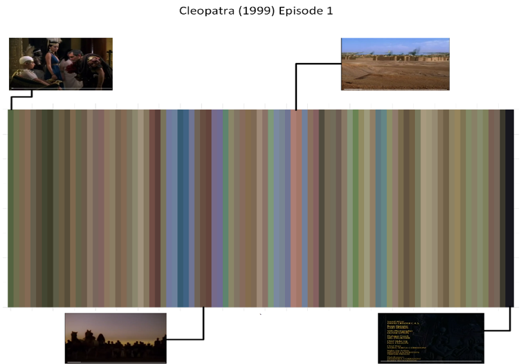
Our initial experiment involves working with a single film, “Cleopatra (Episode 1)” from 1999. In Figure 4, we illustrate the transformation of RGB data into framelines. It’s worth noting that unlike previous tests involving smaller scenes, the framelines in this film exhibit a wider range of distinct colors.
 Figure 4: Framelines for Cleopatra (1999) Episode 1 with 40 seconds capture rate (each line is 40 seconds). Specific scenes and their framelines across the film are shown.
In the previous test case, each frame had predefined labels, making kNN implementation straightforward. However, in the new test case, specific frames lack labels, making kNN implementation more challenging. In this section, we formed clusters of frames, with the cluster size determined arbitrarily. The test set comprises scene splices from the film, with added Gaussian noise.
The clustering model’s accuracy was only 40-50%, which is not practical. Furthermore, with fewer frames, determining the timeslot becomes even more challenging, with accuracy dropping to 10-20% when identifying scene timeslots in the film.
Using a Genomic Data Science Approach: Local Pairwise Alignment
This test case aimed to create an algorithm using local pairwise alignment.
In the field of biology, sequence alignment (DNA, RNA, and proteins) is the process of determining the order and arrangement of nucleotides or amino acids. It helps identify similarities between biological sequences to pinpoint functional or structural regions. There are two primary types of sequence alignment: Global and Local. Furthermore, sequence alignment methods can be categorized based on the number of input sequences: Pairwise alignment and Multiple alignment.
One widely used tool for biological sequencing is BLAST (Basic Local Alignment Search Tool). BLAST compares smaller query sequences (e.g., hundreds of nucleotides) to a vast database of data containing billions of sequences. It identifies subsequences in the database that resemble the queried subsequence.
In summary, this test case focused on creating an algorithm for local pairwise alignment in the context of biological sequence analysis.
For example, querying the nucleotides sequence
ACAGTTAAATTTGTAATTTGGGTTGAGTGAAAACTTCTTTGGGCCTCATACAC AAGCACAGAACCACTAGTTGGGTAGCCTGGCAGTGTCAGAAGTCTGAACCCA GCATAGTGGTCAGCAGGCAGGACGAATCACACTGAATGCAAACCACAGGGTT TCGCAGCGTGGTGAGCATCACCAACCCACAGCCAAGGCGGCGCTGGCTTTTT T
against a database of 2.7 billion nucleotide base pairs of a mouse, according to BLAST, will identify the best alignment at “Mus musculus genome assembly, chromosome 16”.
Sequence alignment, including BLAST, provides valuable insights for building a model to identify specific frames within a film database. Querying nucleotides to a database parallels querying 200 frames to a database with millions of frames. BLAST employs a modified version of the local pairwise alignment algorithm known as the Smith-Waterman algorithm, suitable for comparing sequences of varying lengths.
In DNA sequence alignment, nucleotide sequences consist of characters: G, A, T, and C. In our test case, each frame is represented by characters: R, G, and B, determined by the frame’s maximum value. For example, if the first frame’s maximum value corresponds to red, it is denoted by the character “R.”
 Figure 5: Maximum value of the frames are taken to create a string of characters and then are used with local alignment algorithms to determine the source.
To extract and concatenate to a long string:
largest_col = training_df.Largest_Column.dropna()
largest_colString = largest_col.sum()
largest_colString
GGGGGGGGGGGGGGGGGGGGGGGGGGGRRGGGGGGGGGGGGGGGGGGGG GGGGGGBBRRRRGGGRRRBRRGRRRRRBRBBBRRRRRRRRRRRRRRRRR RRRGGGGGRRRRBRRRRGRRRRRRRRGRGRRRRRRRRRRRRRRRRRRRR RRRRRRRRRRRRRRBBBBBBBRRBBBRBGGGGBBBBBGGRRRRRRRRRR RRRRRRRRRRRRRRRRRRRRRRRR…
In the excerpt displayed above, a notable lack of uniqueness is observed, primarily because the characters ‘R’ and ‘G’ overwhelmingly dominate the concatenated string. When querying a frame using the string “RRRRRRRR,” it results in multiple substrings being identified as the correct alignment. Therefore, it becomes imperative to introduce uniqueness into the process. One viable approach to achieve this uniqueness is by extracting the maximum and minimum RGB columns:
# Find max column
frameline.redux$Largest_Column<-colnames(frameline.redux)[apply(frameline.redux[,1:3],1,which.max)]

# Find min column
frameline.redux$Smallest_Column<-colnames(frameline.redux)[apply(frameline.redux[,1:3],1,which.min)]

#Concat both the max and the min
Next, we mapped the following iterations of the maximum and minimum to a single letter, without rotation:
frameline.redux <- frameline.redux %>%
  mutate(LandSwithrotation = case_when(
    frameline.redux$LandS == "GB" ~ "C",
    frameline.redux$LandS == "BG" ~ "C",
    frameline.redux$LandS == "RG" ~ "Y",
    frameline.redux$LandS == "GR" ~ "Y",
    frameline.redux$LandS == "RB" ~ "P",
    frameline.redux$LandS == "BR" ~ "P",
  ))
training_df = pd.read_csv(path, index_col = None)
long_Seq = training_df.LandSwithrotation.dropna()
long_SeqString = long_Seq.sum()
long_SeqString
An excerpt of the output below show more uniqueness but likewise, still more sparse in uniqueness.
CCCCCCCCCCCPPPPPPPPPCPPPPPPPPPPPCPPCPPPPPPPPPCCYYPC CCPCPCPCCPPPPPPPPPPCYYPPPPPPPPPCCPPPPPPPPPPYCPYYPPPP PPPPYPPPPPPPPPPPPPPPPPPPPPPPPPYPPYPPPPPPPPPPPPPPPPP PPPPPPPPPPPPPPPPPPCPYPCPYPPCYYPPPPPPPPPPPPPPPPPPPPP YPPYPPPPYYPPPCYYYYYPPPPPPPPPPPPPPPPPPPPPPPPPPPPCPPY PYYPPYYPCPCPYPCPPPPPPPPPPPPPPPPPPCPPPPPPCCPCCCCPYYY
If we try the maximum and minimum without rotation, the output delves one level more with uniqueness but is still not enough:
frameline.redux <- frameline.redux %>%
  mutate(LandSwithoutrotation = case_when(
    frameline.redux$LandS == "GB" ~ "C",
    frameline.redux$LandS == "BG" ~ "T",
    frameline.redux$LandS == "RG" ~ "Y",
    frameline.redux$LandS == "GR" ~ "G",
    frameline.redux$LandS == "RB" ~ "P",
    frameline.redux$LandS == "BR" ~ "V",
  ))
long_Seq2 = training_df.LandSwithoutrotation.dropna()
long_SeqString2 = long_Seq2.sum()
long_SeqString2
CCCCCCCCCCCPPPPVPPPPCPPPPPPPPPPPTVVCVPPPPPPPPCCGGPCCCPC PCPCCPPPPPPPPPVTGGPPPPPPPPPCCPPPPPPPPPPYTPGGPPPPPPPPYPP PPPPPPPPPPPPPPVPPPPPPPPYPPYPPPPPPPPPPPPPPPPPPPPPPPPPPPP PPPPPPPCVGVCPGPPTYYPPPPPPPVVPPPPPPPPPPPPYPPYPPPPYYPPPCG GGGYPVVVVVVVVVVVVVVPVVVVVVPPVVVVTVVGVYYVVYYVTVCPGPCPPPP PPPPPPPPPPPPPPTPPPVVVTTVTTTTVGGGGGGVCCGVPPPPPPPPVVPPPVV PPPPPPPPPPPPPPPPPPPPPPPPPPPPYPPPPPYYPPPPPPVVCGVVVVVYVTT TTVPGCPVVVVPYVVTPPPPPPPPPPPPPPVVVVVVVVVPCCYPPPPPYYPYYPT VPPPPPGYPPPPPPCPVVPPPPVPVTVPPPPCPPPPPCVGVCCPVVPPPCCCCCC CCCPPPCPPPPGGCPPPPPPPPPPPCVVVVVVVVVVGGCCCCCCCPPPPPPPPYP VCPPPPPPPPPPPPPPPPPPPPPPPPPPVVGVPPPPPPPPPPPPPPPPPPPPPPP PPPPPPPPPPPPPPPPPPPPPCCPPPPPPPPPPPPPPPPPPPPPGGGCPPVCPVP PPPPPPCPGPVVCGCPPPPPPPPPPPPPPPPPPPPGPPCCTT
The previous examples delves levels deeper into adding uniqueness. If we go beyond the deepest spectrum and use the hexRGB, we get the following excerpt of the output:
#31352F#444A41#3C4339#3D4439#656A5B#777B70#535847#51554C# 444B40#363F32#343E2D#37452C#404F33#3F4334#3F4235#434537#46 4739#444537#424335#6F7A55#839560#849664#78916A#75916B#6077 57#354130#343F31#3C3B34#3E3732#3E413A#454E3D#3E4835#454C35 #454A34#444832#41462F#3C4436#364239#374338#4B5645#8D9077#66 7348#5E6D3E#5E6547#343927#393E2A#3C412B#3D412C#3D422C#3A3F29 #3C412A#3E442C#41472F#444B32#434833#777479#757478#736761#756257#
Next we use Biopython:
aligner = Align.PairwiseAligner()
aligner.mode = 'local'
stringloc = "849664#78916A#75916B#607757#354130#343F31#3C3B34#3E3732#3E413A#454E3D#3E4835#454C35#454A34#444832#41462F#3C4436#"
alignments = aligner.align(stringloc,hexRGBstring)
We can get the highest score, or the subsequence with the greatest likelihood, by using;
alignment = sorted(alignments)[0]
However, my device is limited in memory. Thus, I am unable to continue beyond this part. While I may be unable to pursue the project further due to hardware limitations, I infer that the use of hexRGB may provide excessive uniqueness. Depending on the source, the color schemes of identical frames may vary due to potential issues such as pixel count and resolution disparities.
Conclusion
To complete this project, further research and implementation efforts are necessary, especially sequence alignment.
I am currently waiting to upgrade my PC and hopefully get a GPU to help with the calculations to finish this project. Hopefully by February 2024. {: .notice–info}
Further Study
- Research and implement sequence alignments (Smith-Waterman algorithm) with a better hardware.
- Train using image classification on the framelines: where might a beach/mountain/house scene be in the movie?
- Possible use the image classification to determine if there is a distinct classification of authors or genre.
- A general image classification to determine the name of the film (as seen in the small scenes test case).
- Reduce the capture rate to seconds to increase accuracy in the transformation phase. However, this does increase computation.
Limitations
- Very difficult to find source materials for training and testing due to licensing and legality of films and videos.
- Open source converters are likely to contain malware.
- Imitating the capability of BLAST algorithm is difficult due to limited code available.
