Geometric Brownian Motion on Stock and Option Price Discovery - Matlab

Summary

Quantitative Finance is a field of applied mathematics that employs mathematical and statistical methods to analyze assets. One of the main concepts of quantitative finance is Brownian motion, more specifically Geometric Brownian Motion used in stock price prediction. In this project, GBM was used to model and forecast option contract prices of an asset (specifically Microsoft) with a week-long option contract. Results showed accuracy close to the actual prices albeit to two data points. The probable cause for the inaccuracy may be due to: dividends, examples used were American-style options, and volatility and drift may have been calculated differently. GBM forms the basis of the Black-Scholes equation, the current standard of options pricing today.

Introduction

Brownian Motion is first credited to botanist Robert Brown and decades later, was used by Louis Bachelier to model stock speculation and Albert Einstein to indirectly prove the existence of atoms. The basis of Brownian motion is a random walk, a mathematical model that describes a sequence of steps or movements, where each step is taken randomly and independently of the previous ones. In a one-dimensional random walk, for example, an entity starts at a certain position and, at each time step, moves either to the up or down with some probability. The cumulative effect of these random steps results in a path that exhibits a certain degree of unpredictability and randomness. When time becomes continuous and step size decreases, a random walk equals a Brownian motion. Both concepts are examples of a Markov chain, where future behavior is independent of past history.

Geometric Brownian Motion is defined as when the logarithmic quantity follows a Brownian Motion. GBM is one of the main concepts of quantitative finance for asset price prediction. The log of the Geometric Brownian motion is as follows:

\[log(S_t) = log(S_0) + (\mu - \frac{\sigma^2}{2})t + \sigma W_t\]

where:

$ \mu = $ drift of the stock.

$ \sigma = $ volatility.

$ S_0 = $ initial value/price.

$ S_t = $ forecast price.

$ t = $ small interval time.

$ W_t = $ Wiener process (Normal Distribution).

The drift of the stock, $\mu $, and volatility, $ \sigma $, are the unknown parameters for the equation.

General Steps

The general steps for this project are as follows:

1. Gather Data (NASDAQ).
2. Log(training_data)
3. Calculate the log returns
4. Calculate the drift using the log returns
5. Calculate the variance-covariance matrix using the log returns
6. Use Cholesky Decomposition on the variance-covariance matrix for volatility.

Gathering data

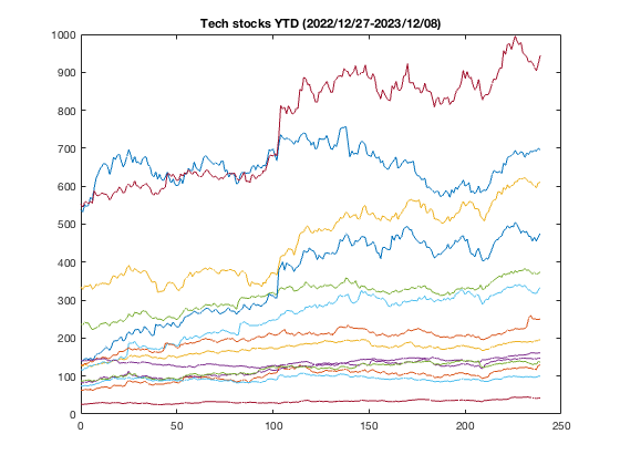
For this project, 14 Tech companies’ stock prices were used. Since the companies are in the same sector (Tech), the prices will be correlated. While data are already adjusted for stock splits and stock consolidation, they do not adjust for dividends. Hence, we will assume that dividends are relatively small and do not affect the overall price of the stock. This is important because even in the Black-Scholes model (discussed later), dividends are assumed to be nonexistent. The 14 Tech companies are as follows: ASML, AMD, AAPL, AMZN, MSFT, META, AVGO, NVDA, CRM, ADBE, IBM, GOOG, TSM, INTC. The stock prices timeframe was from 2022/12/27 - 2023/12/08, one one-day increments.

Once gathering the data, simply log the prices in Matlab:

YTD = log(YTD_dly_price_training);

Calculating drift and volatility

The drift of the stock, $\mu $, and volatility, $ \sigma $, are the unknown parameters for the equation. The drift of the stock is the mean of the returns, which can be calculated by a simple equation: $\frac{1}{T} \sum_{i}^{T} R_t$ where $R_t = \frac{S_t - S_{t-1}}{S_{t-1}}$, such that $S_t$ is the next day log-price, and $S_{t-1}$ is the current day log-price. For volatility, the variance-covariance matrix is calculated from the log returns and subsequently using Cholesky Decomposition. Since the variance-covariance is always symmetric and semi-positive definite, Cholesky Decomposition, $LL^T$, can be used. To get the volatility, we take the diagonal of the resulting $L$. Note that while it is possible to take the standard deviation by the square root of the diagonal of the var-cov matrix, it would leave information about the covariance between the stocks (the whole market movement is ignored).

% log the whole matrix for Brownian motion
YTD = log(YTD_dly_price_training);

% calculate the return
score = diff(YTD)./YTD(1:end-1,:);

%calculate the drift for each column (company)
meanx = mean(score,1);

%calculate volatility
variance = cov(score);
L = chol(variance);
diag_L = diag(L);

Forecasting the Stock Prices

Using the GBM formula with the calculated drift, $\mu $, and volatility, $ \sigma $, we can forecast the price of stocks using multiple simulations. For example, let’s start with forecasting a Monte-Carlo simulation (1000 paths) for the next 5 days (end date is 2023-12-15) for Microsoft:

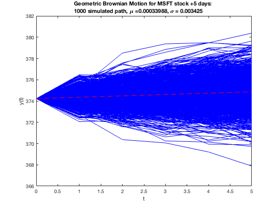
The prices remain stagnant within the 5 days. However, we can see the overall simulations’ possible minimum and maximum values. In a given scenario, an analyst may only include a 95% confidence rate, but here we take the overall 100%. Next, we extend the forecast to +200 days for Microsoft and NVDA.

Left: MSFT vs NVDA +200 days stock prediction

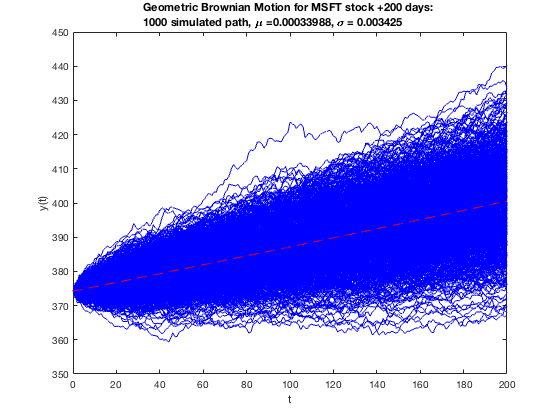
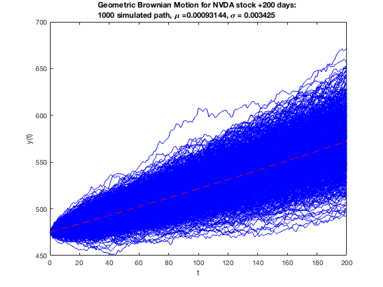
As shown above, the next 200 days of NVDA and MSFT differ. While MSFT is shown to forecast an increase on average \$20, NVDA is poised to increase around \$80. They both have the same volatility, but the values of the mean of returns vary only to the ten-thousands place. If the small value of the drift can have a large impact, so will the volatility. Hence, Cholesky Decomposition’s numerical stability is important when calculating the volatility. Any perturbation causing a slight error up to the ten-thousands place can have a major impact on price prediction.

The following codes are as follows:

%gets the last values
YTD_end = YTD_dly_price_training(end, :);
npaths = 1000; %1000 simulations
stockindex = 5; %Microsoft is the 5th column
r = meanx(stockindex);
day_forecast = 5; %forecast Dec 15 
dicount_factor = exp(-r * day_forecast);
t = (0:1:day_forecast);
y0 = YTD_end(stockindex)*ones(npaths,1);
opts = sdeset('RandSeed', 20231209, 'SDEType', 'Ito');
% function in the SDE toolbox from github
y = sde_gbm(meanx(stockindex), diag_L(stockindex), t, y0, opts);
figure;
plot(t,y,'b',t,y0*exp(r*t),'r--');
xlabel('t');
ylabel('y(t)');
title(['Geometric Brownian Motion for MSFT stock +' int2str(day_forecast) ' days: \newline' int2str(npaths)  ' simulated path, \mu ='   num2str(r) ', \sigma = ' num2str(diag_L(6))])

Note: It is possible to just write a self-owned function using the Geometric Brownian Motion, however, I used a GitHub library already existing due to simplicity and optimization. Here we use SDEtools: https://github.com/horchler/SDETools.

Forecasting the Option Prices

The use of GBM is not directly implemented in stocks but in options. Options is a financial derivative that gives the buyer the right, but not the obligation, to buy an asset for a given price before a predetermined time (expiry). For this project, we take on a Risk Neutral Position (RNP), a position where we ignore the risks, of European-style Options, options that can only be exercised on the expiry date. In an RNP, the drift rate of the stock becomes a risk-free interest rate. Using the same GBM, we can forecast the price of the options per strike price.

Here is a sample of an option contract:

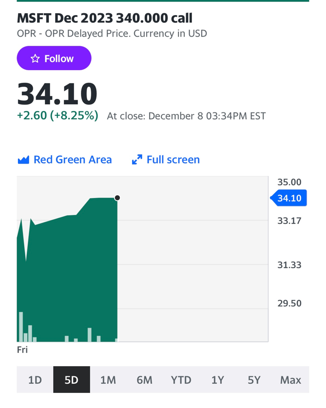
The price of the contract is at \$34.10 for a call option of \$340 for an MSFT option expiring on 2023/12/15.

The code to calculate the difference between the forecasted price and the actual option price:

%December 15 - MSFT option prices for the strike 
%hardcoded since they change over time
strike_prices = [340 342.5 345 347.50 350 352.50 355 357.50 360];

%actual option price per strike price of Microsoft
actual_option_price = [34.10 28.65 29.49 25.85 24.70 21.70 19.79 16.77 15.03];

forecasted_stock = [];
dicount_factor = exp(-r * day_forecast);

% get the forecasted price for each strike price
for i=1:size(strike_prices,2)
    arry_stckprice = strike_prices(i)*ones(npaths,1);
    paystrikes = payoff((y(end,:))',arry_stckprice);
    price = dicount_factor*(sum(paystrikes)/npaths);
    forecasted_stock(end+1) = price;
end

function pay = payoff(S_t, Strikeprice)
    pay = max(S_t-Strikeprice,0);
end

The forecast price was relatively close to the actual price, albeit for two data points, the strike price at \$342.5 and \$347.5 as shown.

Probable cause for this error may be due to:

1. Volatility and Drift may have been calculated differently. For example, drift and volatility may have been calculated using a much bigger data set.

2. We modeled the price using a European-style option but the options in question were American-style options. As each option could have been exercised, the price of the option would have changed.

3. Dividends were assumed to be small. However, in the Black-Scholes model and GBM, assets are assumed to have no dividends.

Black-Sholes Equation

In essence, the following project was a simulation not with GBM but with the Black-Sholes equation. The Black-Scholes equation, developed by economists Fischer Black, Myron Scholes, and Robert Merton in the early 1970s, is a pioneering mathematical model for pricing European-style options. This equation, a partial differential equation, takes into account factors such as the current stock price, the option’s strike price, the time to expiration, the risk-free interest rate, and the underlying asset’s volatility. The Black-Scholes model provides a theoretical framework for estimating the fair market value of options

Limitations

Geometric Brownian Motion (GBM) is a widely used model in finance, particularly in the context of option pricing, but it comes with several limitations that can affect its accuracy in capturing market dynamics for option price discovery:

1. Constant Volatility and Drift: GBM assumes constant volatility and drift over time. In reality, these parameters often change, especially during periods of market turbulence. The model fails to capture the volatility clustering observed in real financial markets.

2. Normal Distribution of Returns: GBM assumes that stock returns are normally distributed. However, empirical evidence suggests that stock returns exhibit fat tails and skewness, meaning extreme events occur more frequently than a normal distribution would predict.

3. Market Frictions: The GBM model does not account for transaction costs, taxes, or other market frictions. In reality, these factors can significantly impact option prices and trading strategies.

4. Risk-Neutral Assumption: The model is based on the assumption of risk neutrality, meaning that investors are indifferent to risk. In practice, investors often exhibit risk aversion, especially during times of uncertainty, leading to deviations from the model’s predictions.

5. Continuous Time Assumption: GBM operates in continuous time, assuming that prices change continuously. In reality, financial markets operate in discrete time, with prices changing in intervals. Discrepancies between continuous-time models like GBM and the actual market behavior can impact option pricing accuracy.

6. Non-Stationary Trends: GBM assumes a stationary process, meaning that statistical properties do not change over time. Financial markets, however, exhibit non-stationary trends, making it challenging for GBM to capture evolving market conditions accurately.

7. Lack of Jumps: GBM does not incorporate price jumps, which are abrupt and large movements in asset prices. In reality, jumps occur, especially during significant news events or market shocks, and their absence in the model can lead to inaccuracies in option pricing. The jumps are “discontinuous” points, which are prevalent in stock market movements. It is one of the early critics of using the GBM as a model for price speculation.

8. Assumption of Log-Normality: GBM assumes that the underlying asset’s price follows a log-normal distribution. This assumption may not always hold, particularly in the presence of extreme market events.

Gamestop

An example of this is Gamestop:

As shown, the price jump in January 2021 is very unpredictable and improbable for GBM and Black-scholes to predict. This movement caused huge financial losses to market makers and option sellers.

Conclusion

GBM forms the basis of the Black-Scholes equation, the current standard of options pricing today. GBM and Black-Scholes are a simplification of a complex financial system. For example, stock prices are non-stationary time series, with changing volatility and drift. Likewise, GBM and Black-Scholes are incapable of forecasting unpredictable events in the real world. Lastly, with the increased use of High-Frequency Trading (HFT) for price discovery, quantitative finance is becoming more dominant in the current market, increasing speculation. The recent increase in speculation has likewise increased volatility, which has been considered to be one cause of the recent recessions. The current state of quantitative finance is the application of machine learning, however, whether it improves the state of the market is still questionable.