
Nyc Parking Violations
Parking Violations in NYC FY23
Description
The following dataset was derived from: https://data.cityofnewyork.us/City-Government/Parking-Violations-Issued-Fiscal-Year-2023/pvqr-7yc4 . For each fiscal year, the number of citations will have more thn 15-20 million rows. The FY23 only contains about 3 million data rows due the fiscal year starting in July 1st, 2022.
Load Libraries
#if(!require("sf")) install.packages("sf")
#if(!require("leaflet")) install.packages("leaflet")
#if(!require("tigris")) install.packages("tigris")
#if(!require("httr")) install.packages("httr")

library(tidyverse)
library(dplyr)
library(lubridate)
library(ggrepel)
library(sf)
library(osmdata)
library(tidygeocoder)
library(httr)
library(rgdal)
library(broom)
library(rlang)
library(ggplot2)
Import Dataset
The following data set has been download at the time of October 8,2022. Any new updates will not be reflected on the data set.
parking_violations_FY23 <- read.csv("Parking_Violations_Issued_-_Fiscal_Year_2023.csv")Descriptions
The data set has 3133085 and 43 columns/features.
The features description are:
| Source Column Name | Description/Comment |
|---|---|
| SUMMONS-NUMBER | UNIQUE IDENTIFIER OF SUMMONS |
| PLATE ID | REGISTERED PLATE ID |
| REGISTRATION STATE | STATE OF PLATE REGISTRATION |
| PLATE TYPE | TYPE OF PLATE |
| ISSUE-DATE | ISSUE DATE |
| VIOLATION-CODE | TYPE OF VIOLATION |
| SUMM-VEH-BODY | VEHICLE BODY TYPE WRITTEN ON SUMMONS (SEDAN, ETC.) |
| SUMM-VEH-MAKE | MAKE OF CAR WRITTEN ON SUMMONS |
| ISSUING-AGENCY | ISSUING AGENCY CODE |
| STREET-CODE1 | GEOGRAPHICAL STREET CODE |
| STREET-CODE2 | GEOGRAPHICAL STREET CODE |
| STREET-CODE3 | GEOGRAPHICAL STREET CODE |
| VEHICLE EXPIRATION | DATE VEHICLE EXPIRATION DATE ON SUMMONS |
| VIOLATION LOCATION | GENERAL VIOLATION LOCATION |
| VIOLATION PRECINCT | PRECINCT OF VIOLATION |
| ISSUER PRECINCT | PRECINCT OF ISSUANCE |
| ISSUER CODE | UNIQUE CODE IDENTIFYING ISSUING OFFICER |
| ISSUER COMMAND | COMMAND OF ISSUING OFFICER |
| ISSUER SQUAD | ISSUING OFFICER’S SQUAD |
| VIOLATION TIME | TIME VIOLATION OCCURRED |
| TIME FIRST OBSERVED | TIME OF INITIAL VIOLATION OBSERVATION |
| VIOLATION COUNTY | COUNTY OF VIOLATION |
| FRONT-OF-OPPOSITE | VIOLATION IN FRONT OF OR OPPOSITE |
| HOUSE NUMBER | ADDRESS NUMBER OF VIOLATION |
| STREET NAME | STREET NAME OF SUMMONS ISSUED |
| INTERSECTING STREET | VIOLATION NEAR INTERSECTING STREET |
| DATE FIRST OBSERVED | DATE OF INITIAL VIOLATION OBSERVATION |
| LAW SECTION | SECTION OF VEHICLE & TRAFFIC LAW |
| SUB DIVISION | SUB DIVISION ON SUMMONS IMAGE |
| VIOLATION LEGAL CODE | TYPE OF LEGAL CODE |
| DAYS IN EFFECT | DAYS PARKING IN EFFECT |
| FROM HOURS IN EFFECT | START TIME POSTED FOR METER AND SIGN VIOLATIONS |
| TO HOURS IN EFFECT | END TIME POSTED FOR METER AND SIGN VIOLATIONS |
| VEHICLE COLOR | CAR COLOR WRITTEN ON SUMMONS |
| UNREGISTERED VEHICLE? | UNREGISTERED VEHICLE INDICATOR |
| VEHICLE YEAR | YEAR OF VEHICLE WRITTEN ON SUMMONS |
| METER NUMBER | PARKING METER NUMBER FOR METER VIOLATIONS |
| FEET FROM | NUMBER OF FEET FROM CURB FOR HYDRANT VIOLATION |
| VIOLATION POST CODE | LOCATION POST CODE OF VIOLATION |
| VIOLATION DESCRIPTION | DESCRIPTION OF VIOLATION |
| NO STANDING OR STOPPING | VIOLATION SUMMONS INDICTOR FOR NO STANDING OR STOPPING |
| HYDRANT VIOLATION SUMMONS | INDICATOR FOR HYDRANT VIOLATION |
| DOUBLE PARKING VIOLATION | SUMMONS INDICATOR FOR DOUBLE PARKING VIOLATION |
Parking Violations based on Date-Times
Preprocessing
Before we begin the following analysis, it is important to preprocess the dataset to reflect the current fiscal year 2023. New York City fiscal year begins on July 1st of each year and ends on June 30th of the following year. Hence the FY2023 began in July 1, 2022 and will end in June 30th 2023. However, the following data set has parking violation issue dates that are misrepresented as other years. Hence, it is important to remove the misrepresented years in the data set first.
First we change the Report Date to date format and create a new column for years.
temp_parking_violations_FY23 <- parking_violations_FY23 %>%
  mutate(`Issue.Date` = mdy(parking_violations_FY23$`Issue.Date`)) %>%
  mutate(`Issue.year` = as.factor(year(`Issue.Date`))) %>%
  select(`Issue.year`)
As show below. There are years not issued within the Fiscal year of 2023.
table(temp_parking_violations_FY23)## temp_parking_violations_FY23
## 2000 2012 2014 2017 2018 2019 2020 2021 2022 2023
## 9 3 1 1 1 2 38 347 3132474 157
## 2024 2025 2026 2027 2028 2029 2031 2049 2066
## 12 6 1 24 2 3 2 1 1The next step is to filter the data set within the Fiscal year time frame 2022-06-01 to the time of when the data set was downloaded [2022-10-08].
new_parking_violations_FY23 <- parking_violations_FY23 %>%
  mutate(`Issue.Date` = mdy(parking_violations_FY23$`Issue.Date`),
         `Issue.weekday` = wday(`Issue.Date`, label=TRUE)) %>%
  filter(`Issue.Date` >= mdy("06/01/2022") & `Issue.Date` <= mdy("10/08/2022"))

cat("The new dimension of the data set: \n");dim(new_parking_violations_FY23)
## The new dimension of the data set:## [1] 3131197 44Furthermore we convert the feature Violation.Time to a date_time. For example, the following data populates the feature: 1037A, 1205P, 1052A. We can infer that the A represents AM and P represents PM.
We can use lubdridate parse_date_time code IMp to convert the timestamp. However, it requires that A -> AM, and P -> PM. Hence, we will add concatenate M to the end of the strings.
#Convert the time using parse_date_time
new_parking_violations_FY23 <- new_parking_violations_FY23 %>%
  mutate(Violation.Time = str_c(Violation.Time, "M"),
         Violation.Time = parse_date_time(Violation.Time, "IMp", tz="EST"),
         Violation.Time.Hour = hour(Violation.Time))

#str(new_parking_violations_FY23$Violation.Time.Hour)
Parking violations vs dates Analysis
We will create a bar plot of the parking violations issue by dates, as shown below:
violations_by_date <- new_parking_violations_FY23 %>%
  count(`Issue.Date`, sort=TRUE) %>%
  ggplot() +
  geom_col(mapping = aes(x=`Issue.Date`, y = n)) +
  labs(title = "Number of violations per day")
violations_by_date
We would expect the violations to be higher in the summer, but it seems that the violations issues remain consistent in the 4 months of data. This may be attributed that most tourist in the summer do not drive into NYC. Likewise, the data for October may be absent if the previous month data is only uploaded at the first of the next month. We may not see October data until the start of November.
Parking Violations vs weekdays
Next we analyze the difference by weekday:
violations_by_weekday <- new_parking_violations_FY23 %>%
  count(`Issue.weekday`) %>%
  ggplot() +
  geom_col(mapping=aes(x=`Issue.weekday`, y=n))
violations_by_weekday
During the weekdays (M-F), the number of violations is higher than in the weekends. This may be due to the work week, where more people are moving.
Parking by Hours (EST)
violations_by_hour <- new_parking_violations_FY23 %>%
  count(`Violation.Time.Hour`) %>%
  ggplot() +
  geom_line(mapping = aes(x=`Violation.Time.Hour`, y=n))
violations_by_hour
The majority of the violations occur during 9pm - 3pm, which may be due to the work hours.
Parking Violations based on Vehicle data
Parking Violations by Registraton state
violations_by_registration_state <- new_parking_violations_FY23 %>%
  count(`Registration.State`, sort=TRUE) %>%
  head(10) %>%
  ggplot() +
  geom_col(mapping = aes(x=reorder(`Registration.State`, -n), y = n)) +
  labs(title = "Parking violations by Registrations")  +
  theme(axis.text.x = element_text(angle=90, v=.2))
violations_by_registration_state
Not surprisingly, a majority of the violations are New York held license plate. However, there are other registered license plate not from New York, especially Florida. We can only assume these cars are from tourists.
Parking Violations by Make
violations_by_make <- new_parking_violations_FY23 %>%
  count(`Vehicle.Make`, sort=TRUE) %>%
  head(5) %>%
  arrange((`Vehicle.Make`))  %>%
  mutate(freq = round((n/sum(n) * 100), digits=4)) %>%
  mutate(cs = rev(cumsum(rev(freq))),
         pos = freq/2 + lead(cs,1),
         pos = if_else(is.na(pos), freq/2, pos))
graph_violations_by_make <- violations_by_make %>%
ggplot(mapping=aes(x="", y=freq, fill=`Vehicle.Make`)) +
geom_col() +
geom_label_repel(aes(label=paste0(freq, "%"), y=pos),
force=.5, nudge_x = .5, nudge_y = .5) +
coord_polar(theta="y") +
labs(title="Percentage of Violations by the top 5 makes Makes")
graph_violations_by_make
Toyota and Honda are the most popular car to have violations.
Parking Violations by Manufactured Years of top 5 Makes
We filter some vehicles misrepresented as manufactured beyond 2024. Note that car manufactures releases the next year cars around the summer. For example, a Nissan Altima 2023 may come out on the summer of 2022. WE discretize the values into the folowing ranges: pre-1990, 1991-2000, 2001-2010, 2011-2020, 2021+
#Discretize into ranges
to_graph_violations <- new_parking_violations_FY23 %>%
  filter(`Vehicle.Make` %in%  violations_by_make$`Vehicle.Make`,
         `Vehicle.Year` < 2024 & `Vehicle.Year` != 0)  %>%
  mutate(`Discretized.Year` = case_when(
           between(`Vehicle.Year`, 1970, 1990) ~ "pre-1990",
           between(`Vehicle.Year`, 1991, 2000) ~ "1991-2000",
           between(`Vehicle.Year`, 2001, 2010) ~ "2001-2010",
           between(`Vehicle.Year`, 2011, 2020) ~ "2011-2020",
           between(`Vehicle.Year`, 2021, 2023) ~ "post-2021",
           TRUE ~ NA_character_)) %>%
  count(`Vehicle.Make`, `Discretized.Year`, sort= TRUE) %>%
  ggplot(aes(fill=`Discretized.Year`)) +
  geom_bar(aes(x=`Vehicle.Make`, y = n), stat="identity") +
  theme(axis.text.x = element_text(angle=90, v=.2)) +
  labs(title="Top 5 Vehicle makes by Vehicle year")

to_graph_violations
A majority of the violations are from each of the top 5 makes is from cars manufactured 2011-2020.
Parking Violations by Plate
most_issued_car <- new_parking_violations_FY23 %>%
  count(`Plate.ID`, sort=TRUE) %>%
  head(10)
most_issued_car
A majority of normal individuals have zero to a few violations in a span of their lifetime However, these top 9 License plate have hundreds of citations/violations already in a span of 4 months! Repeated crime breakerss…..
Parking violations based on Violation Code and Issuer Agency
There are over 100 violations codes listed. We examine the top 10 violations:
top_10_violations <- new_parking_violations_FY23 %>%
  count(`Violation.Code`, sort=TRUE) %>%
  head(10)
top_10_violations
Top 10 violations and their respective names and fines according to NYC:
| Violation.Code | Violation Description | Violation Fine Amount ($) |
|---|---|---|
| 5 | BUS LANE VIOLATION | 50 |
| 7 | FAILURE TO STOP AT RED LIGHT | 50 |
| 14 | NO STANDING-DAY/TIME LIMITS | 115 |
| 20 | NO PARKING-DAY/TIME LIMITS | 60-65 |
| 21 | NO PARKING-STREET CLEANING | 45-65 |
| 36 | PHTO SCHOOL ZN SPEED VIOLATION | 50 |
| 38 | FAIL TO DSPLY MUNI METER RECPT | 35-65 |
| 40 | FIRE HYDRANT | 115 |
| 70 | REG. STICKER-EXPIRED/MISSING | 65 |
| 71 | INSP. STICKER-EXPIRED/MISSING | 65 |
We filter the following top 10 violations and get the top 5 Issuing Agencies.
top_5_agency <- new_parking_violations_FY23 %>%
  filter(Violation.Code  %in%  top_10_violations$Violation.Code) %>%
  count(`Issuing.Agency`, sort=TRUE) %>%
  head(5)
top_5_agency
The following top 5 issuing agencies and their respective names:
- K-PARKS DEPARTMENT
- P-POLICE DEPARTMENT
- S-DEPARTMENT OF SANITATION,
- T-TRAFFIC,
- V-DEPARTMENT OF TRANSPORTATION,
Then, we create a stack chart of the top 10 violations and top 5 issuing agencies.
to_graph <- new_parking_violations_FY23 %>%
  filter(Violation.Code  %in%  top_10_violations$Violation.Code) %>%
  filter(Issuing.Agency  %in%  top_5_agency$Issuing.Agency) %>%
  mutate(Violation.Code = as.factor(Violation.Code)) %>%
  count(Issuing.Agency,Violation.Code) %>%
  ggplot(aes(fill=`Violation.Code`)) +
  geom_bar(aes(x=Issuing.Agency, y = n), stat="identity") +
  theme(axis.text.x = element_text(angle=90, v=.2)) +
  labs(title="Top 10 violations with the top 5 agencies that issues them")
to_graph
The Department of Transportation issues the most violations, a majority of which are vehicles speeding on a school zone caught by cameras!
Parking Violations based on Location Data
Data pre-processing
The goal of this section is to create a mapped data of the parking violations in NYC. However, this is a major undertaking due to the lack of latitude and longitude features in the dataset. The parking violations have locations, but is represented into three different features: House.Number, Street.Name, Intersecting.Street.
An example output of the three features:
geocode_NYC <- new_parking_violations_FY23 %>%
  select(House.Number, Street.Name, Intersecting.Street) %>%
  head(10)
geocode_NYC
As shown, if the violation occurred in-front of a house or building, it is possible to combine House.Number and Street.Name to find the general location. However, if the violation occurred in the intersection, House.Number will be most likely be empty, only giving us the intersecting streets (Street.Name and Intersecting.Street ), which may be difficult to convert to a general location of latitude and longitude data.
For simplicity (and ease), we only consider the locations with given House.Number, Street.Name, Violation County. We will use Violation County because it will narrow our search to a particular county when using the function geocoder later.
Selecting just the House.Number, Street.Name, Violation County:
geocode_NYC_house.street <- new_parking_violations_FY23 %>%
  select(House.Number, Street.Name, Violation.County)
head(geocode_NYC_house.street,4)
As seen above, unfortunately, some data in House.Number, Street.Name, or Violation County may be empty (""), not NA.
We need to remove the empty cells ("") belonging to both feature:
geocode_NYC_house.street <- geocode_NYC_house.street[geocode_NYC_house.street$House.Number != "",]
geocode_NYC_house.street <- geocode_NYC_house.street[geocode_NYC_house.street$Street.Name != "", ]
geocode_NYC_house.street <- na.omit(geocode_NYC_house.street)
print("As shown below, the new data set:")
## [1] "As shown below, the new data set:"head(geocode_NYC_house.street,5)The dataset was cleaned for missing values, reducing our dimension to:
dim(geocode_NYC_house.street)## [1] 1673269 3From the step above, Violation County was not cleaned for any missing data or misrepresented values. The approach to Violation County is different. As shown below, the unique values of Violation County:
unique(geocode_NYC_house.street$Violation.County)## [1] "NY" "BX" "K" "" "Q" "R" "MS" "Kings" "Qns"
## [10] "Bronx" "Rich" "QNS"Among the different values that Violation.County can represent, these are the most important to consider to help us geocode the addresses:
K abd Kings = Brooklyn
BX and Bronx = Bronx
NY = NY
Q and QNS = Queens
R, Rich = Staten Island
We filter and recode the different unique values of Violation County into their respective true names:
#Discretize the test set to be used for later problem

#geocode_NYC_house.street_Manhattan to map Manhattan later
geocode_NYC_house.street_Manhattan <- within(geocode_NYC_house.street,
                      {
                      County <- NA
                      County[Violation.County == "NY"] <- "NY"
                      }) %>%
  na.omit()

#geocode_NYC_house.street to map the 5 counties with map overlay
geocode_NYC_house.street <- within(geocode_NYC_house.street,
                      {
                      County <- NA
                      County[Violation.County == "NY"] <- "NY"
                      County[Violation.County == "BX" | Violation.County == "Bronx"] <- "Bronx"
                      County[Violation.County == "K" | Violation.County == "Kings"] <- "Brooklyn"
                      County[Violation.County == "Rich" | Violation.County == "R"] <- "Staten Island"
                      County[Violation.County == "QNS" | Violation.County == "Q"] <- "Queens"
                      }) %>%
  na.omit()
Due to filtering the data set, the new dimension is:
dim(geocode_NYC_house.street)## [1] 1652703 4We can confirm that we only have the 4 counties in interest:
unique(geocode_NYC_house.street$County)## [1] "NY" "Bronx" "Brooklyn" "Queens"
## [5] "Staten Island"The next step is to combine the following House.Number, Street.Name, and County into a single column to be used for geocoding. Likewise, “raw” duplicated Full_Address values are removed.
full_geocode_address <- geocode_NYC_house.street %>%
  mutate(Street = str_c(House.Number, Street.Name, sep=" "),
         County_State = str_c(County, "NY" , sep=","),
         Full_Address = str_c(Street, County_State, sep = ",")) %>%
  select(Full_Address) %>%
  distinct(Full_Address)
Unfortunately, we cannot differentiate between different lemmatized values. For example, Washington Square may be present in the data set as Washington SQ or Washington Square. Otherwise, the “raw” distinct have reduced our data set.
The concatenated dataset now looks:
head(full_geocode_address,5)The new dimension:
dim(full_geocode_address)## [1] 367777 1Geocoding
Geocoding is the process of converting the street addressing to physical longitude and latitude data. In this step, we process the address that was created from the above steps
Important Note: Everything in this section can implemented easier if the library ggmap did not rely on Google API Query to get information. Unfortunately, to request geocode in ggmap requires a register GOOGLE API Key, which requires Billing($$).
The library tidygeocoder provides a geocoding function through Querying the United States Census Bureau(https://geocoding.geo.census.gov). However, unlike the Google API Query, the Census Bureau is limited to process a batch of 10,000. It also requires no API Key!.
Hence, to batch:
# The batch limit is 10,000 for Census Bureau
batchsize <- 10000
groups <- ceiling(nrow(full_geocode_address)/batchsize)

#We split it into n groups
fils <- split(full_geocode_address, factor(sort(rank(row.names(full_geocode_address))%%groups)))
After creating the batch list needed for query, we will now apply it to geocode. Since it only accepts tibbles, we create a list of tibbles and apply the function:
get_lat_long <- function(Full_Address) {
  tmp <- tibble(Full_Address)
  tmp <- tmp %>%
    tidygeocoder::geocode(address =Full_Address, method = "census", verbose = FALSE)
}
Using lapply to recursively unpack the list of list and apply the above function.
Important Note: Since this requires batching queries, it takes a lot of time to iterate and retrieve data, hence we will eval = FALSE this chunk so we don’t have to rerun it again. We save the result as a csv and read it again to save time. Every 10,000 batch on average took 4-5 minutes. Hence, 50 bacthes can take up to 3-4 hours for every rerun!
#retrives Longitude and latitude
newLongandLat <- lapply(fils, lapply, get_lat_long)

# Flatten the list of tibbles to a single list and bind them:
flat_location <- bind_rows(flatten(newLongandLat))

#Not all location will return a long and lat due to data error
flat_location <- na.omit(flat_location)

# Write to csv
write.csv(flat_location, "NYC_longitude_latitude.csv", row.names = FALSE)
Read the output csv file:
flat_csv_long_lat <- read.csv("NYC_longitude_latitude.csv")Ensure that the long and lat are within respective longitude and latitude ranges of New York City:
flat_csv_long_lat <- flat_csv_long_lat %>%
  filter(`long` >= -75.0 & `long` <= -73.0,
         `lat` >= 40.4 & `lat` <=  41.0)
The dim of the long_lat
dim(flat_csv_long_lat)## [1] 258010 3After geocoding the data set now has longitude and latitude data:
head(flat_csv_long_lat,10)Downloading the New York City Shapefile
As mentioned earlier, the library ggmap would make a lot of steps simpler if it did not require a registered GOOGLE API KEY (which requires paying for the service). One alternative method is to download the New York city shapefiles:
Note: since the AWS Access Key expires, query the following html and copy that into the code. The hard coded query will change per each rerun.
# If rerunning, query the following address in the browser and copy the resulting address into map <- readOG()
# ('http://data.beta.nyc//dataset/0ff93d2d-90ba-457c-9f7e-39e47bf2ac5f/resource/35dd04fb-81b3-479b-a074-a27a37888ce7/download/d085e2f8d0b54d4590b1e7d1f35594c1pediacitiesnycneighborhoods.geojson')

map <- rgdal::readOGR("https://data-beta-nyc-files.s3.amazonaws.com/resources/35dd04fb-81b3-479b-a074-a27a37888ce7/d085e2f8d0b54d4590b1e7d1f35594c1pediacitiesnycneighborhoods.geojson?Signature=VxZ1OST93MNZN1e4V7se6haki2A%3D&Expires=1666721574&AWSAccessKeyId=AKIAWM5UKMRH2KITC3QA")
## OGR data source with driver: GeoJSON
## Source: "https://data-beta-nyc-files.s3.amazonaws.com/resources/35dd04fb-81b3-479b-a074-a27a37888ce7/d085e2f8d0b54d4590b1e7d1f35594c1pediacitiesnycneighborhoods.geojson?Signature=VxZ1OST93MNZN1e4V7se6haki2A%3D&Expires=1666721574&AWSAccessKeyId=AKIAWM5UKMRH2KITC3QA", layer: "OGRGeoJSON"
## with 310 features
## It has 4 fieldsFinal Map
nyc_neighborhoods_df <- tidy(map)
ggplot() +
  geom_polygon(data=nyc_neighborhoods_df, aes(x=long, y=lat, group=group)) +
  geom_point(data=flat_csv_long_lat, aes(x=long, y = lat), alpha = 1/20, size=.0001, color = "red") +
  theme_void()
We can see to the right side, Queens County, having very sparse data points. This can be attributed to the fact that Queens County makes up from other smaller ‘Neighborhoods’. For example, [147-20 Cherry Ave, Flushing, NY] is in Queens County but Flushing Neighborhood. Unlike the other four counties, we cannot standardize Queens County as [Full Address, Queens, NY] because it will return a lat and long of NA. For example, [147-20 Cherry Ave, Queens, NY] will return NA, even if it belongs in Queens County.
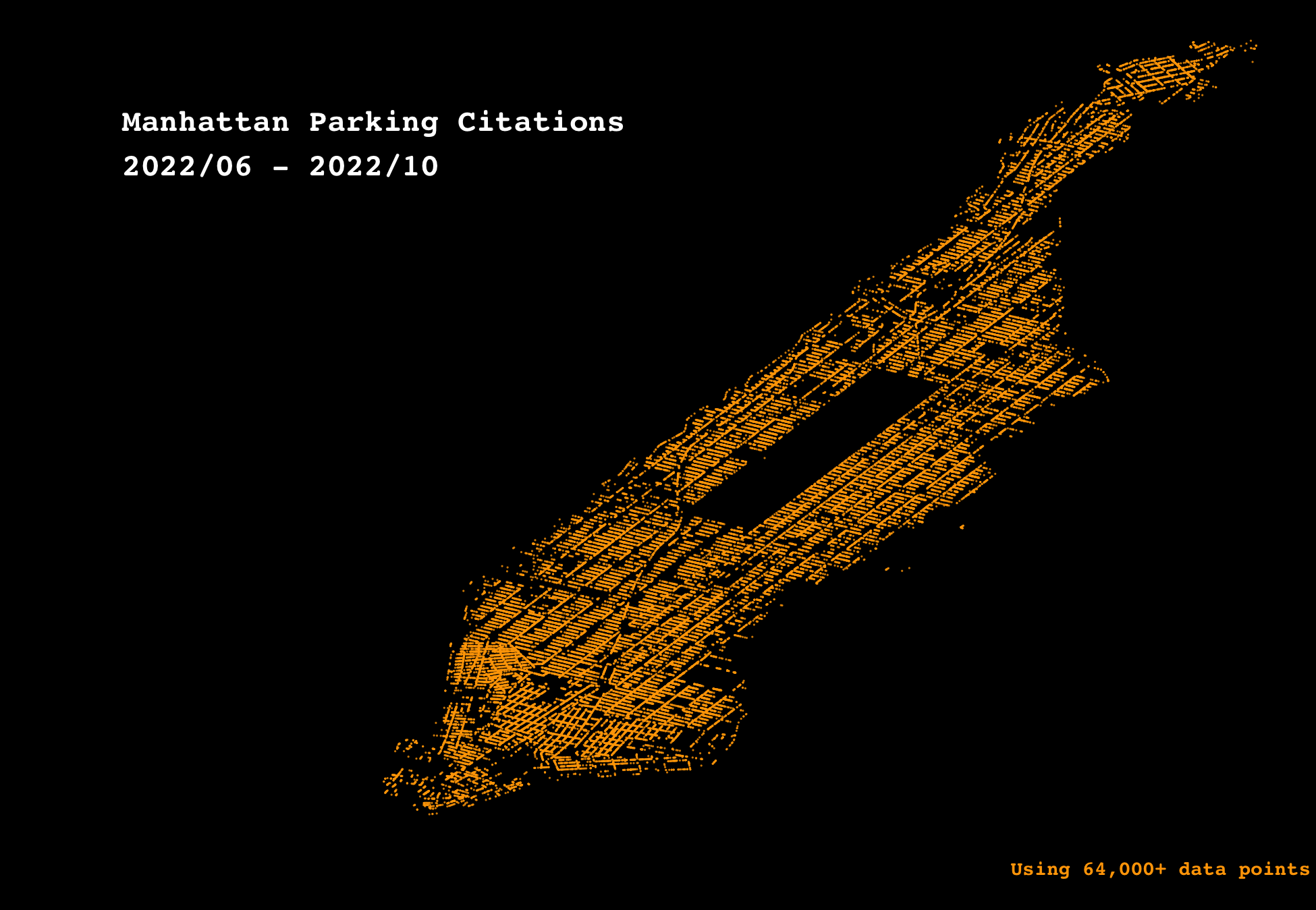
Mapping Manhattan using Point w/o map overlay
In this section, we focus on mapping Manhattan County only without the map overlay.
Read the output csv file:
Manhattan_geocode <- flat_csv_long_lat[grep("NY,NY", flat_csv_long_lat$Full_Address), ]Ensure that the long and lat are within respective longitude and latitude ranges of New York City:
Manhattan_geocode <- Manhattan_geocode %>%
  filter(`long` >= -75.0 & `long` <= -73.0,
         `lat` >= 40.4 & `lat` <=  41.0)
The dim of the long_lat
dim(Manhattan_geocode)## [1] 64146 3After geocoding the data set now has longitude and latitude data:
head(Manhattan_geocode,10)# For centering the ggplot
min_long <- min(Manhattan_geocode$long) + .06
max_long <- max(Manhattan_geocode$long)
min_lat <- min(Manhattan_geocode$lat) + .05
max_lat <- max(Manhattan_geocode$lat)
# Plot the following points
ggplot() +
geom_point(data=Manhattan_geocode, aes(x=long, y = lat), alpha = .8, size=.03, shape = 16, color = "orange")+
scale_y_continuous(limits=c(min_lat,max_lat)) +
scale_x_continuous(limits=c(min_long,max_long)) +
annotate("text", x= -74.05, y = 40.85, label = "Manhattan Parking Citations \n2022/06 - 2022/10", col = "white", family = "mono", fontface="bold", hjust=0) +
annotate("text", x= max_long-.03, y = min_lat, label = "Using 64,000+ data points", col = "orange", family = "mono", fontface="bold", hjust=0, size=2.5) +
theme_void()+
theme(panel.background=element_rect(fill='black'))
#ggsave("manhattan.png")We can almost map out all of the streets in Manhattan!
Mapping Brooklyn using Point w/o map overlay:
brooklyn_geocode <- flat_csv_long_lat[grep("Brooklyn,NY", flat_csv_long_lat$Full_Address), ]dim(brooklyn_geocode)## [1] 133018 3#For centering ggplot
min_long <- min(brooklyn_geocode$long)
max_long <- max(brooklyn_geocode$long)
min_lat <- min(brooklyn_geocode$lat)
max_lat <- max(brooklyn_geocode$lat) - .10
#plot the given points
ggplot() +
geom_point(data=brooklyn_geocode, aes(x=long, y = lat), alpha = .8, size=.03, shape = 16, color = "orange")+
scale_y_continuous(limits=c(min_lat,max_lat)) +
annotate("text", x= min_long , y = max_lat, label = "Brooklyn Parking Citations \n2022/06 - 2022/10", col = "white", family = "mono", fontface="bold", hjust=0) +
annotate("text", x= max_long-.05, y = min_lat, label = "Using 130,000+ data points", col = "orange", family = "mono", fontface="bold", hjust=0, size=2.5) +
theme_void() +
theme(panel.background=element_rect(fill='black'))
#ggsave("Brooklyn.png")Tidygeocoder
Since the batch querying was done once to reduce the time for reruns, here is an example of the output of tidygeocoder with small data:
examples_address <- tibble(line_address= c("1700 CROTONA AVE,Bronx,NY", "82 UNION ST,Brooklyn,NY", "99 EARHART LN,Bronx,NY"))
examples_address <- examples_address %>%
    tidygeocoder::geocode(address = line_address, method = "census", verbose = TRUE)
##
## Number of Unique Addresses: 3## Executing batch geocoding...## Batch limit: 10,000## Passing 3 addresses to the US Census batch geocoder## Querying API URL: https://geocoding.geo.census.gov/geocoder/locations/addressbatch## Passing the following parameters to the API:## format : "json"## benchmark : "Public_AR_Current"## vintage : "Current_Current"## Query completed in: 1.2 secondsexamples_addressFurther Improvement:
As discussed earlier, geocoding the address is a computationally expensive task. It will be more expensive if we scale up the project to a billion points. Suppose we want to aggregate all parking tickets post 2010, the amount of data to process will be expensive. However, the map will be more visually appealing; we can map out Manhattan with more density!
There are other implementations that connects the ticket to the “centreline” of the given city and then compute the centroid of the street. The computation is more efficient but does not compute the exactness.
Likewise, we avoided using Intersection between two street names. Tidygeocoder has the capability of mapping intersection. However, after several experiments, batch encoding with method = “census” did not work as expected with the given dataset (it may work better with other dataset). I was only able to get about 5-10% to return a lat and long through batch encoding. Using method = “arcgis” provide superior results by giving a lat and long, but does not support batch encoding. Using arcgis would be computationally expensive even if it allows us to create a more “completed visualized map”.