Description
This report investigates ploice incidents recorded by the Norfolk Police Department that occurred over the last five years (2017-2022). The following data set was derived at: https://data.norfolk.gov/Public-Safety/Police-Incident-Reports/r7bn-2egr
Load Libraries
library(tidyverse)
library(dplyr)
library(lubridate)
library(sf)
library(tidygeocoder)
library(httr)
library(ggplot2)
library(gganimate)
library(tigris)
library(rlang)
Import Dataset
nrfk_police_incident <- read.csv("https://data.norfolk.gov/api/views/r7bn-2egr/rows.csv?accessType=DOWNLOAD")The dimension of the following data set:
dim(nrfk_police_incident)## [1] 114540 12Preprocessing
Removing empty data values from the dataset:
nrfk_police_incident <- nrfk_police_incident[nrfk_police_incident$Block.Address != "",]
nrfk_police_incident <- nrfk_police_incident[nrfk_police_incident$Street != "", ]
nrfk_police_incident <- na.omit(nrfk_police_incident)
The dataset was cleaned for missing values, reducing our dimension to:
dim(nrfk_police_incident)## [1] 107183 12The next step is to combine the following Block.Address and Street into a single column to be used for geocoding. County and State is padded to create a Full_Address Value as discussed in the previous project in NYC Parking Violations.
full_geocode_address <- nrfk_police_incident %>%
  mutate(Street = str_c(Block.Address, Street, sep=" "),
         Full_Address = str_c(Street, "Norfolk, VA", sep = ",")) %>%
  select(-c(Block.Address, Street))
Likewise, to batch:
# The batch limit is 10,000 for Census Bureau
batchsize <- 10000
groups <- ceiling(nrow(full_geocode_address)/batchsize)

#We split it into n groups
split <- split(full_geocode_address, factor(sort(rank(row.names(full_geocode_address))%%groups)))
Next, a function is created to geocode the Full_Address Values feature. Unlike the previous project, we will use both census and arcgis methods to create a more complete mapping. The function geocode_combine in tidygeocoder will allow us to use the method= arcgis if the return value in method = census is NA. Census allows for batch encoding but may result in NA values, hence arcgus (which lacks batching) is used soon after.
get_lat_long <- function(addr) {
  tmp <- tibble(addr)
  print(tmp)
  tmp <- tmp %>%
    tidygeocoder::geocode_combine(
      queries = list(
        list(method = "census"),
        list(method = "arcgis")
      ),
      global_params = list(address = 'Full_Address')
    )
}
Apply the function to the list:
#retrieves Longitude and latitude
newLongandLat <- lapply(split, get_lat_long)

# Flatten the list of tibbles to a single list and bind them:
flat_location <- bind_rows(flatten(newLongandLat))

#Not all location will return a long and lat due to data error
#flat_location <- na.omit(flat_location$Full_Address)

# write to a csv to reduce rerun
write.csv(flat_location, "NorfolkPoliceIncident.csv", row.names = FALSE)
Read the output csv file:
flat_csv_long_lat <- read.csv("NorfolkPoliceIncident.csv")Ensure that the following Norfolk City map box and transform the date-time:
flat_csv_long_lat <- flat_csv_long_lat %>%
  filter(`long` >= -76.5 & `long` <= -76.0,
         `lat` >= 36.8 & `lat` <=  37.5) %>%
  mutate(`Date.of.Occurrence` = mdy(`Date.of.Occurrence`),
         `Year.of.Occurrence` = int(year(`Date.of.Occurrence`)))
Data Visualization
Heatmap
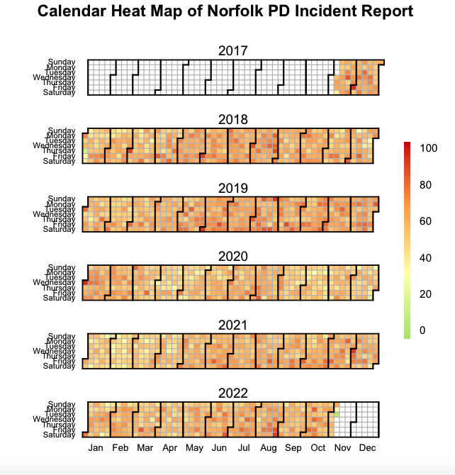
We create a calendar series heatmap. We use the following function called calendarHeat() using Paul Bleicher function: https://github.com/iascchen/VisHealth/blob/master/R/calendarHeat.R
heatmap_incident <- flat_csv_long_lat %>%
  count(Date.of.Occurrence)

# calendar heat map
calendarHeat(heatmap_incident$Date, heatmap_incident$n, varname="Norfolk PD Incident Report", color = "g2r")
Point Maps
As seen form the previous project in NYC, we can map out the total number of incidents:
ggplot() +
  geom_point(data=flat_csv_long_lat, aes(x=long, y = lat), alpha = .8, size=.03, shape = 16, color = "orange") +
  theme_void() +
  theme(panel.background=element_rect(fill='black'))
However, unlike NYC, the points are more sparse. This may be attributed to being a suburban city rather than a compact city like NYC or Washington D.C.
Number of Incidents per year:
Let’s examine yearly changes in the incident rates in Norfolk.
ggplot() +
  geom_point(data=flat_csv_long_lat, aes(x=long, y = lat, color = factor(Year.of.Occurrence )), alpha = .8, size=.5, shape = 16, show.legend = FALSE) +
  theme_void() +
  theme(panel.background=element_rect(fill='black')) +
  transition_time(Year.of.Occurrence) +
  labs(title='Year: {frame_time}') +
  ease_aes("linear")

anim_save("YearofOccurence.gif")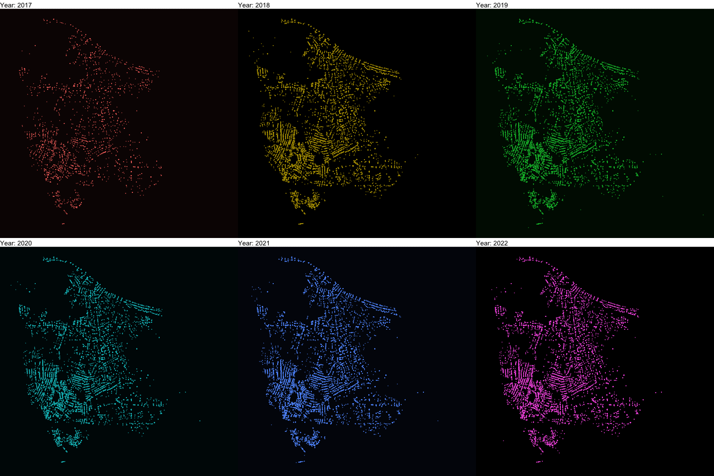
It is colorful just in time for the holiday season, but does not tell us meaning full information.
Crime rate
Next, we examine the top 5 Offenses:
top_offense <- flat_csv_long_lat %>%
  count(Offense, sort = TRUE) %>%
  head(5)
top_offense
## Offense n
## 1 HIT & RUN - PROPERTY 12734
## 2 LARCENY - FROM AUTO 11561
## 3 VANDALISM 10965
## 4 SIMPLE ASSAULT 6307
## 5 DOMESTIC-SIMPLE ASSAULT 5625As shown, Hit & Run, Larceny, and Vandalism, and Simple Assaults(2) accounts for the top 5 Offenses in Norfolk.
#we filter the dataset to only contain the top 5
by_offense <- flat_csv_long_lat %>%
  filter(Offense %in% top_offense$Offense) %>%
  count(Offense,Year.of.Occurrence)

p <- ggplot() +
  geom_line(data = by_offense, mapping = aes(x = Year.of.Occurrence, y = n, group = Offense, color = Offense)) +
  labs(title = "Top 5 offenses over the years")

ggsave("OffenseByYear.png")

#add gganimate animations
p + transition_reveal(Year.of.Occurrence)
anim_save("OffenseByYear.gif")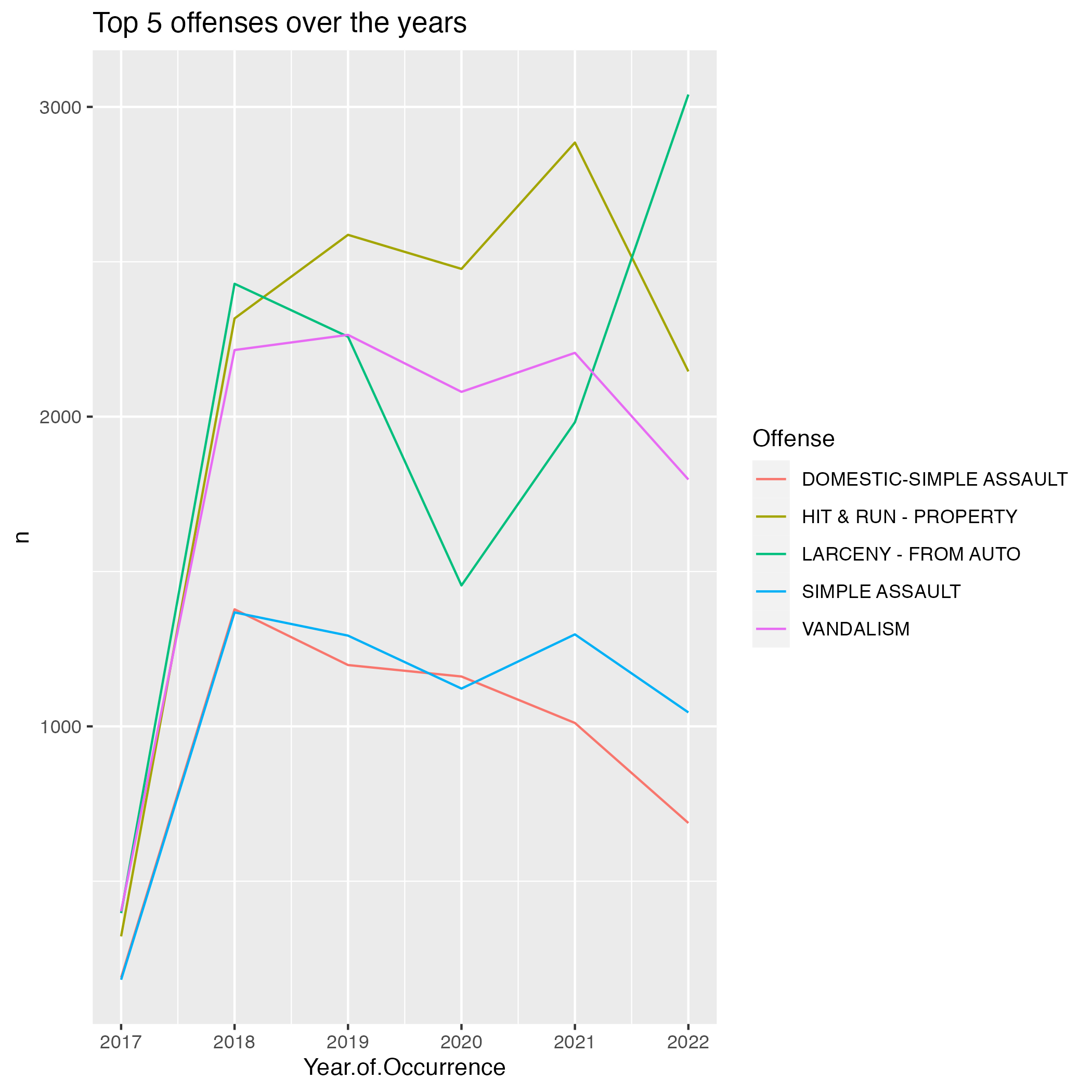
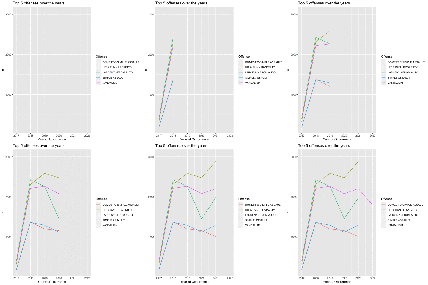
4 of the top 5 offense surprisingly decreased coming into 2022. However, there is a sharp rise in Larcency - from Auto.
Mapping top locations of crime across Norfolk
Next, we examine the top locations of crime across Norfolk.
First we create the base map for Norfolk using tigris since I did not find an appropriate shapefile for Norfolk.
nrfk_tract <- tracts(state = "51", county ="710")

# get the water area since its included in the boundary for norfolk
water = area_water(state = "51", county ="710")
Finally, we overlap the top 50 crime areas over time into the base map:
# get the top 50 crime areas
by_offense_lat_long <- flat_csv_long_lat %>%
  count(lat, long, sort = TRUE) %>%
  head(50)

# standardized the pallete of all 50 "color" for ggplot
standardize = rep('red', times = 50)

# creating the plot
by_offense_lat_long_year <- flat_csv_long_lat %>%
  filter(flat_csv_long_lat$long %in% by_offense_lat_long$long & flat_csv_long_lat$lat %in% by_offense_lat_long$lat ) %>%
  count(lat, long, Year.of.Occurrence) %>%
  mutate(`lat.long` = str_c(lat,long)) %>%
  ggplot() +
  geom_sf(data=nrfk_tract) +
  geom_sf(data =water , fill = "black", color = NA, aes(geometry = geometry)) +
  theme_void() +
  theme(panel.background=element_rect(fill='black')) +
  coord_sf(xlim = c(-76.34557,-76.17),
           ylim = c(36.82076,36.98)) +
  geom_point(aes(x=long, y = lat, size = n, color = lat.long), alpha = .5, show.legend =  FALSE) +  scale_size(range=c(1,15)) +
  scale_color_manual(values = standardize) +
  transition_time(Year.of.Occurrence) +
  labs(title='Top 50 crime areas in Norfolk, Year: {frame_time}') +
  ease_aes("linear")

#by_offense_lat_long_year

anim_save("OffenseByMap.gif")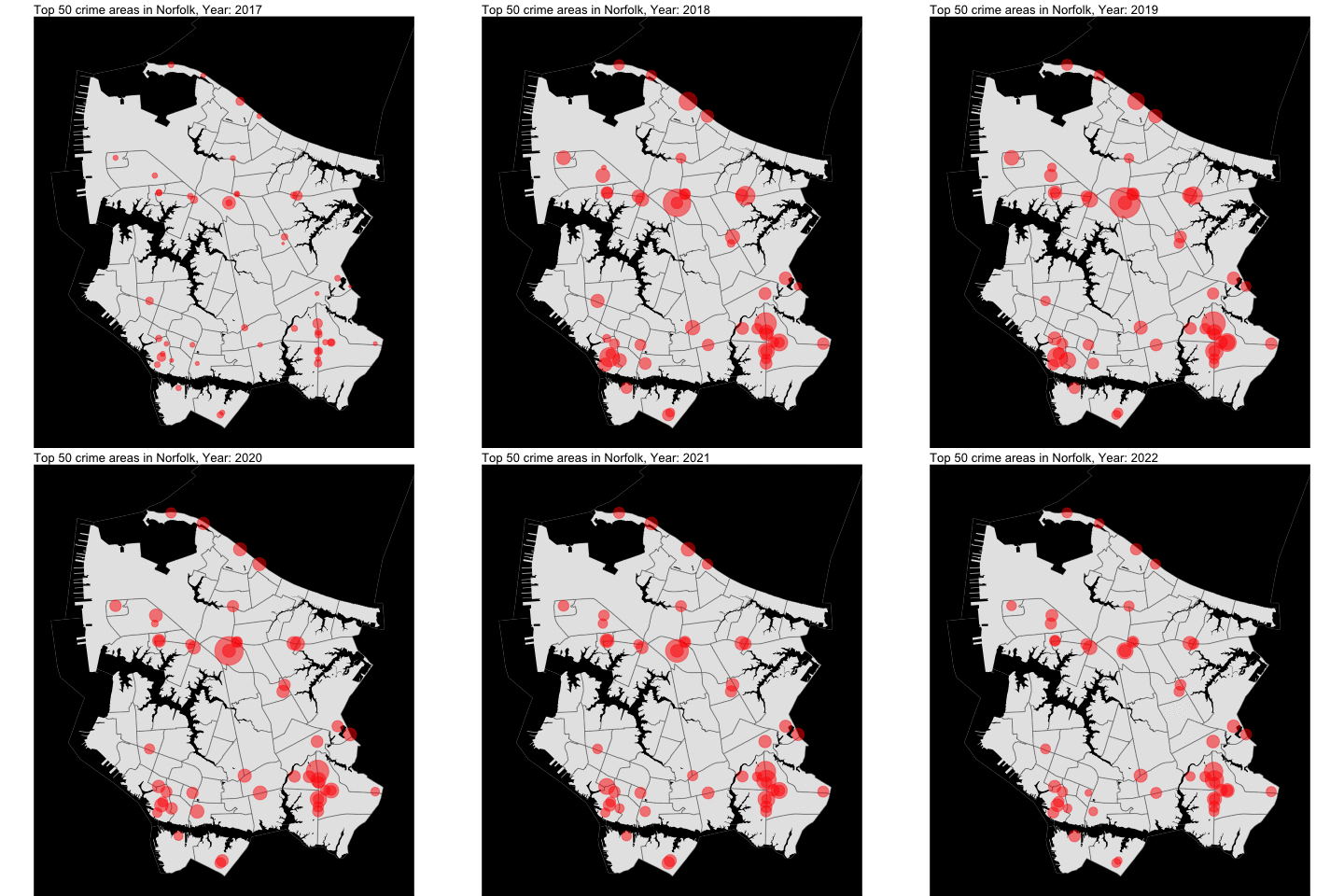
As someone who lived in Norfolk for two decades, the areas that I picked in the map are Military Circle Mall area, Downtown Norfolk, and Tidewater (close to Walmart!)!!!
The top 10 of these locations are located at:
by_address <- flat_csv_long_lat %>%
  count(`Full_Address`, sort = TRUE)%>%
  head(10)
by_address
## Full_Address n
## 1 7500 TIDEWATER DR,Norfolk, VA 1162
## 2 1200 MILITARY HWY,Norfolk, VA 1018
## 3 800 MILITARY HWY,Norfolk, VA 637
## 4 5900 VIRGINIA BEACH BLVD,Norfolk, VA 613
## 5 1100 MILITARY HWY,Norfolk, VA 561
## 6 7500 TIDEWATER DRIVE,Norfolk, VA 502
## 7 900 LITTLE CREEK RD,Norfolk, VA 423
## 8 7500 GRANBY ST,Norfolk, VA 375
## 9 1800 LITTLE CREEK RD,Norfolk, VA 356
## 10 6400 CRESCENT WAY,Norfolk, VA 342
