Linear Regression Introduction
Building this page….
Intro
Linear Regression attempts to model the relationship between variables by fitting a linear equation.
Dataset
The data used in this project are simple dimensional inputs for those learning the fundamentals of linear regression. Suppose we have the data set: inputs X=[-1. -0.8 -0.6 -0.4 -0.2 0 0.2 0.4 0.6 0.8 1] and the corresponding outputs Y=[-5.4 -4.9 -4.5 -3.6 -2.7 -2. -1.1 -0.1 0.1 1.1 1.5]. Suppose we need to find the linear regression function $y=w_1x+w_0$ according to the regularized least square method. That is, solve the following minimization problem:
\(\min_{w_0,w_1}F(w_0,w_1)=\sum_{j=1}^{11} (w_1x_j +w_0 - y_j)^2 + \mu (w_0^2+w_1^2),\)
where $\mu=0.1$.
We first initialize the inputs and the outputs.
X = np.array([-1, -0.8, -0.6, -0.4, -0.2, 0, 0.2, 0.4, 0.6, 0.8, 1])
Y = np.array([-5.4, -4.9, -4.5, -3.6, -2.7, -2, -1.1, -0.1, 0.1, 1.1, 1.5])
N=X.shape[0]
mA=np.array([np.ones(N),X])
mA=np.transpose(mA)

#The result of mA should be similar to the expected 'A' matrix for our formula:
#[[ 1.  -1. ]
# [ 1.  -0.8]
# [ 1.  -0.6]
# [ 1.  -0.4]
# [ 1.  -0.2]
# [ 1.   0. ]
# [ 1.   0.2]
# [ 1.   0.4]
# [ 1.   0.6]
# [ 1.   0.8]
# [ 1.   1. ]]
Next we solve the following equation:
$\nabla F(w) = 2A^T(Aw-y) $
Set $ \nabla F(w)=0$ to solve the minimizer \((A^T A )w^*=A^T y\) or $w^* = (A^T A)^{-1}A^T y$ (see How)
from numpy import linalg as lu
# use x=LA.solve(A,b) to solve Ax=b
mu=0.1
mA_t=np.transpose(mA)
mI=np.eye(2) # generate the 2x2 idenity matrix, or use np.identity(mA.shape[1])
vw_st=lu.solve(mA_t@mA + mu*mI, mA_t@Y)
which will give us w* = [-1.94594595 3.59555556] or in other words, w0 = -1.94594595 and w1 = 3.59555556.
Calculating F(w*)
Recall that: \(F(w)=\|Aw-y\|_{\ell^2}^2 + \mu \|w\|_{\ell^2}^2\)
In Python we can represent it like:
ssq = np.sum((mA@vw-Y)**2) + mu*(np.sum(vw**2))
print('F(w_0*,w_1*): ',ssq)
Which should result in: F(w*): 2.151478678678679
Using Gradient descent method to find the approximate minimizer.
That is to solve the following equation:
\[(w^{k+1}_0,w^{k+1}_1)=(w^k_0,w^k_1) - \eta \nabla F(w^k_0,w^k_1)\]
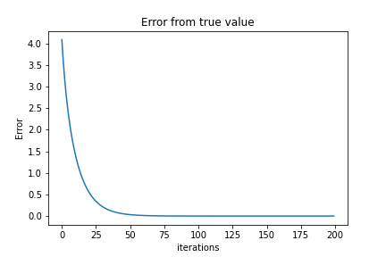
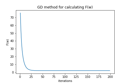
We can include F(w) for each iteration to check if we converge to the real answer we found ‘analytically’ above (F(w*)). Our stopping criterion is N number of iterations (another stopping criterion would be to introduce an error). In this example, $ \eta $ , or the learning rate, is set to .01.
f_X = lambda __w: 2*(np.transpose(mA@__w)-Y)@mA + mu*2*(np.transpose(__w))

w_k = np.zeros([200,2])
#print(w_k)
iter_N = 200 % We will run this part for 200 iterations
gradF = 0
eta = .01
fn = np.zeros(iter_N) #reserve the array slots

for __ in range (1,iter_N):  #we start at 1 since 0 is already initialize
    gradF = f_X(w_k[__-1])
    w_k[__] = w_k[__-1] - eta*gradF
    fn[__] =np.sum((mA@w_k[__]-Y)**2) + mu*(np.sum(w_k[__]**2))


print(w_k[-1,:])
print(fn[-1]
The last value for the array fn should result in approximately the same value found in F(w*), showing us that the gradient descent method is correct. As for the last value of wk, it should be approximate to [-1.94594595, 3.59555553].


